|
|
You are here: Foswiki>Software/FastJets Web>WholeEventQjets (24 Apr 2012, GeorgJahn)Edit Attach
t-tbar-Reconstruction Based on Partitioning
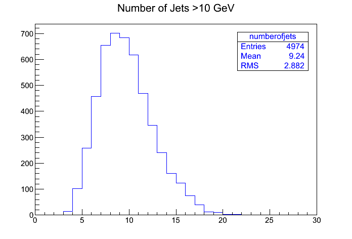 The average 14 TeV t-tbar-event from Pythia clustered with anti-kt (0.7) has about 9 jets with p_T over 10 GeV (pruned or unpruned does not matter), 99% of the events have 4-18 jets. The idea of partitioning is to divide these jets into three partitions, we will call them top1, top2 and others; the jets of the first two partitions are supposed to "belong" to one of the produced tops and jets in the others-partition should be those jets that are not related to the t-tbar-production.To find the "correct" partition, one could implement several algorithms which try to reconstruct the tops via searching for sets of jets that are likely to have been a top ( positive approach) or which or which try to eliminate unlikely combinations ( negative approach). Note that these algorithms do rely on the assumption that a "correct" partition exists and that jets really belong to either one of the either one of the tops or not tho them at all.
The amount of possible partitions into 3 subsets of a set with n entries is 3^n. As we do not care about which top is which, the number of possibilities is reduced to the sum of i = 1 to n over (2^(i-1)-1)*n!/i!/(n-i)! which already takes into account that the two top sets shall not be empty and which can easily be simplified to 1/2 * 3^n - 2^n + 1/2. This is still in the order of magnitude of 1/2*3^n and thus growing exponentially with n. For the average n=9 jets, this gives 9.330 possibilities, for our upper bound of n=18 it gives about 2 * 10^8 possibilities, the average over all n as they appear in our collisions being about 10^7 possibilities. Since this is for pratical purposes often too high, it is here suggested to skip any events with n>=18, which gives us an average 1.2 * 10^6 combinations, while just omitting 0.7% of the events. Other possibilities follow in the table below:
The average 14 TeV t-tbar-event from Pythia clustered with anti-kt (0.7) has about 9 jets with p_T over 10 GeV (pruned or unpruned does not matter), 99% of the events have 4-18 jets. The idea of partitioning is to divide these jets into three partitions, we will call them top1, top2 and others; the jets of the first two partitions are supposed to "belong" to one of the produced tops and jets in the others-partition should be those jets that are not related to the t-tbar-production.To find the "correct" partition, one could implement several algorithms which try to reconstruct the tops via searching for sets of jets that are likely to have been a top ( positive approach) or which or which try to eliminate unlikely combinations ( negative approach). Note that these algorithms do rely on the assumption that a "correct" partition exists and that jets really belong to either one of the either one of the tops or not tho them at all.
The amount of possible partitions into 3 subsets of a set with n entries is 3^n. As we do not care about which top is which, the number of possibilities is reduced to the sum of i = 1 to n over (2^(i-1)-1)*n!/i!/(n-i)! which already takes into account that the two top sets shall not be empty and which can easily be simplified to 1/2 * 3^n - 2^n + 1/2. This is still in the order of magnitude of 1/2*3^n and thus growing exponentially with n. For the average n=9 jets, this gives 9.330 possibilities, for our upper bound of n=18 it gives about 2 * 10^8 possibilities, the average over all n as they appear in our collisions being about 10^7 possibilities. Since this is for pratical purposes often too high, it is here suggested to skip any events with n>=18, which gives us an average 1.2 * 10^6 combinations, while just omitting 0.7% of the events. Other possibilities follow in the table below:
| skip on |
events omitted |
average # of partitions |
| n>=20 | 0.1% | 3.2 * 10^6 |
| n>=18 | 0.7% | 1.2 * 10^6 |
| n>=16 | 3% | 3.2 * 10^5 |
| n>=14 | 8.5% | 7.5 * 10^4 |
The Negative Approach
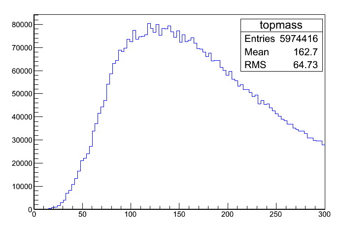
For the negative approach one has to think of observables that are anticipated to have certain values for the "correct" or at least a "likely" reconstruction and that have a different distribution of values for random partitions. A good example for this is the invariant mass of top1 and top2 which results from simply adding the four-momenta of the jets and calculating the invariant mass of the resulting four-vector.Invariant Mass
 As we can see very clearly, the reconstructed (=correct) partitions have a highly different mass distribution from random partitions. For this and the following plots a reconstruction algorithm was chosen that tries to reconstruct the partitions based on the knowledge of the four-momenta of the created tops. The algorithm is not perfect and might have flaws, but is still useful for the comparisons in the next part. One still has to be careful and keep in mind, that the algorithm may have problems and the distributions might not be exactly true. Because of the reconstruction process the reconstructed distribution (blue) is not as perfect as the masses of the underlying pythia tops (green), but it is blurred by inaccuracies. (Note: A "perfect" algorithm seems impossible because of the ill-definedness of the correct reconstruction and the large amount of times where no reasonable reconstruction can be found. The chosen algorithm rejects 50% of the events because they do not seem to have likely reconstructions.)
So, for example, when requiring the mass to be 130 GeV < m < 210 GeV, one can filter out about 5/6 of the possible combinations (red) while barely loosing any correct reconstructions. (Smaller mass-ranges seem to make more sense and give a better ratio.) Still, we assume a top mass here, which is often the thing that we want to determine.
As we can see very clearly, the reconstructed (=correct) partitions have a highly different mass distribution from random partitions. For this and the following plots a reconstruction algorithm was chosen that tries to reconstruct the partitions based on the knowledge of the four-momenta of the created tops. The algorithm is not perfect and might have flaws, but is still useful for the comparisons in the next part. One still has to be careful and keep in mind, that the algorithm may have problems and the distributions might not be exactly true. Because of the reconstruction process the reconstructed distribution (blue) is not as perfect as the masses of the underlying pythia tops (green), but it is blurred by inaccuracies. (Note: A "perfect" algorithm seems impossible because of the ill-definedness of the correct reconstruction and the large amount of times where no reasonable reconstruction can be found. The chosen algorithm rejects 50% of the events because they do not seem to have likely reconstructions.)
So, for example, when requiring the mass to be 130 GeV < m < 210 GeV, one can filter out about 5/6 of the possible combinations (red) while barely loosing any correct reconstructions. (Smaller mass-ranges seem to make more sense and give a better ratio.) Still, we assume a top mass here, which is often the thing that we want to determine. 
Mass Difference
To solve this, one can look at the observable deltaM := |m_top1 - m_top2| which should be "small" for correct reconstrutions. The plot below shows us that indeed, this is a useful observable for discrimination: A cut at deltaM < 50 GeV would filter out 89.5% of the random possibilities while including 98.5% of all correct partitions. Even lower cuts cut make sense. Thus, the mass difference is one of the most helpful observables. Note that the reconstructed distribution is obviously shifted to the right compared to the Pythia-distribution, because of blurring effects. .Angle Between the Tops
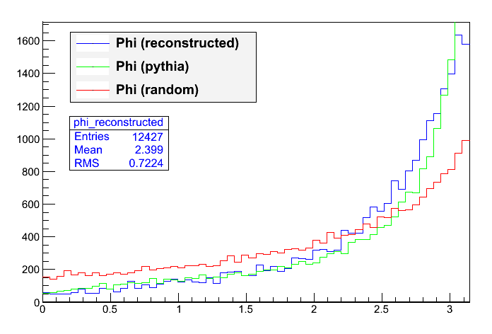 One would also expect that the angle phi between the two tops in the transverse plane is rather high. The plot to the right illustrates this, the red distribution displays once again the random partitions, whereas the blue distribution is a reconstruction and the green shows the ideal behavior from Pythia. Once again, the reconstruction is not as "sharp" as the ideal top phi distribution. Even though the jets are picked out at random (red), still, they are likely to be back to back, since the overall event is nearly balanced and only one third on average of the jets is in the others-partition. It seems that phi is thus not very good for discrimination, so only low cuts on phi should make sense, e.g. phi > 1 filters out 16.5% of the random partitions, but also about 7% of the reconstructed combinations.
Still, it is not clear, if a cut on this variable does make much sense at all since it could introduce systematic errors.
.
.
One would also expect that the angle phi between the two tops in the transverse plane is rather high. The plot to the right illustrates this, the red distribution displays once again the random partitions, whereas the blue distribution is a reconstruction and the green shows the ideal behavior from Pythia. Once again, the reconstruction is not as "sharp" as the ideal top phi distribution. Even though the jets are picked out at random (red), still, they are likely to be back to back, since the overall event is nearly balanced and only one third on average of the jets is in the others-partition. It seems that phi is thus not very good for discrimination, so only low cuts on phi should make sense, e.g. phi > 1 filters out 16.5% of the random partitions, but also about 7% of the reconstructed combinations.
Still, it is not clear, if a cut on this variable does make much sense at all since it could introduce systematic errors.
.
.
Transverse Momentum Sum of the Tops
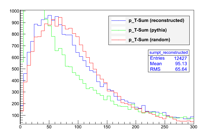 Let us look at the p_T-Sum defined as | p_T_top1 + p_T_top2 | (vector addition), which is a similar observable to phi, but takes into account more information. We can see that in this case, the distribution from the reconstructed tops does not look very different than the distribution from random partitions. Once again, this is because the whole event is nearly balanced and only about one third of the jets is – in average – in the others-partition. Still, the ideal distribution looks different, but not different enough to make a discrimation cut very effective.
In this scenario, neutrino events were considered as normal events, but even, if one only looks at hadronic decays, one will find very similar distributions for the reconstructed and random partitions. In a nutshell, the p_T-sum does not seem to be a reasonable observable for discrimination.
.
Let us look at the p_T-Sum defined as | p_T_top1 + p_T_top2 | (vector addition), which is a similar observable to phi, but takes into account more information. We can see that in this case, the distribution from the reconstructed tops does not look very different than the distribution from random partitions. Once again, this is because the whole event is nearly balanced and only about one third of the jets is – in average – in the others-partition. Still, the ideal distribution looks different, but not different enough to make a discrimation cut very effective.
In this scenario, neutrino events were considered as normal events, but even, if one only looks at hadronic decays, one will find very similar distributions for the reconstructed and random partitions. In a nutshell, the p_T-sum does not seem to be a reasonable observable for discrimination.
.
Jet Count per Top
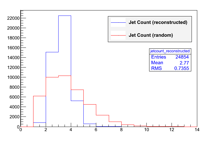 A very simple observable is the jet count, i.e. the number of jets that are combined to one top. Obviously, the random partitions follow a smoothened binomial distribution here, whereas the reconstructed partitions should consist of 2-3 jets. This is demonstrated in the plot: As presumed, the number of jets is usually between 2 and 4. The enormous amounts of higher possibilities are very seldom, thus it seems resonable to introduce a cut of either n<6 or even n<5, the latter filtering out 35.5% of the random combinations, but only about 2.5% of the correct partitions.
A cut of n>1 is a bit worse, as it filters out 3.5% of the right combinations, but 27.5% of the random combinations. (This may appear to contradict the plot, but the cut was always chosen such that both top partitions are required to fulfill the constraint, whereas the plot shows the individual numbers.)
.
A very simple observable is the jet count, i.e. the number of jets that are combined to one top. Obviously, the random partitions follow a smoothened binomial distribution here, whereas the reconstructed partitions should consist of 2-3 jets. This is demonstrated in the plot: As presumed, the number of jets is usually between 2 and 4. The enormous amounts of higher possibilities are very seldom, thus it seems resonable to introduce a cut of either n<6 or even n<5, the latter filtering out 35.5% of the random combinations, but only about 2.5% of the correct partitions.
A cut of n>1 is a bit worse, as it filters out 3.5% of the right combinations, but 27.5% of the random combinations. (This may appear to contradict the plot, but the cut was always chosen such that both top partitions are required to fulfill the constraint, whereas the plot shows the individual numbers.)
.
Jet Collimation
 The idea of the next observable is the fact that the contributing jets for a top are likely to point in the same direction. For this purpose, the standard deviation from the contributing jets' directions in the transverse plane was calculated.
The plot illustrates that the behaviour is as expected, the reconstructed partitions are more collimated (except from the partitions which only consist of one single jet, where a deviation of 0 is assumed). Still, the distributions are not so different, that a cut would be very useful.
.
.
.
The idea of the next observable is the fact that the contributing jets for a top are likely to point in the same direction. For this purpose, the standard deviation from the contributing jets' directions in the transverse plane was calculated.
The plot illustrates that the behaviour is as expected, the reconstructed partitions are more collimated (except from the partitions which only consist of one single jet, where a deviation of 0 is assumed). Still, the distributions are not so different, that a cut would be very useful.
.
.
.
Conclusion
 Due to the vast amount of possible partitions, one would need to combine several cuts to eliminate the massive background: Initially, the background to signal ratio would be about 10^7 to 1. Even with a very hard cuts in all the reasonable observables above, this ratio could not be lowered to something acceptable. There was no cut combination found which was able to make the signal clearly visible on the background. Though this is also mathematically obvious, it is also illustrated with a mass distribution plot. Ten thousand random partitions of ten thousand events that fulfilled the following cuts were entered into the plot: deltaMass < 20, phi > 1, 1 < jetCount < 5. No top mass peak is visible. Note, that about 1-10 correct partitions would be expected – a quantity obviously not recognizable in the vast amount of entries.
Since "hard" cuts give no visible result whatsoever, it is expected, that also smooth cuts in the QJets-sense (weight-functions based on the observables) will not be able to extract the signal based on the above-named observables. Nevertheless, many different possibilities based on a gaussian weight function exp(-x*x*alpha*alpha) have been explored. The rigidity factor alpha is chosen such that 1/alpha is in the order of magnitude of the original cut parameter. Two of these plots are shown below, both with a weight depending on delta mass, as this seems to be the most interesting observable. The plot to the left has a moderate alpha of 1/20 where als the plot to the right has a higher alpha of 1/7.
Due to the vast amount of possible partitions, one would need to combine several cuts to eliminate the massive background: Initially, the background to signal ratio would be about 10^7 to 1. Even with a very hard cuts in all the reasonable observables above, this ratio could not be lowered to something acceptable. There was no cut combination found which was able to make the signal clearly visible on the background. Though this is also mathematically obvious, it is also illustrated with a mass distribution plot. Ten thousand random partitions of ten thousand events that fulfilled the following cuts were entered into the plot: deltaMass < 20, phi > 1, 1 < jetCount < 5. No top mass peak is visible. Note, that about 1-10 correct partitions would be expected – a quantity obviously not recognizable in the vast amount of entries.
Since "hard" cuts give no visible result whatsoever, it is expected, that also smooth cuts in the QJets-sense (weight-functions based on the observables) will not be able to extract the signal based on the above-named observables. Nevertheless, many different possibilities based on a gaussian weight function exp(-x*x*alpha*alpha) have been explored. The rigidity factor alpha is chosen such that 1/alpha is in the order of magnitude of the original cut parameter. Two of these plots are shown below, both with a weight depending on delta mass, as this seems to be the most interesting observable. The plot to the left has a moderate alpha of 1/20 where als the plot to the right has a higher alpha of 1/7.

 .
.
.
.
.
.
.
.
.
.
.
.
.
.
.
.
.
.
.
.
.
.
Simplified Approach
 To simplify the previous efforts, in the next section, we only take a look at the jets that are a direct result of the t-tbar-decay. The plot to the right shows that these are only about 4-7 jets, which corresponds to 2-4 jets per produced top. Sometimes, jets may overlap, so that only three jets or two are visible, but this is not the usual case. The lower number of jets also decreases the number of possible partitions by several orders of magnitude. In average, there are now only about 10^3 possible partitions per t-tbar-decay (calculated by the formula above). This can still be reduced, as we know, that all of the jets should be included into either the top1 or the top2 partition, which leaves us with only 2^(n-1) partitions, i.e. less than 50 possible combinations in average.
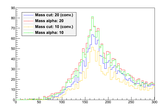
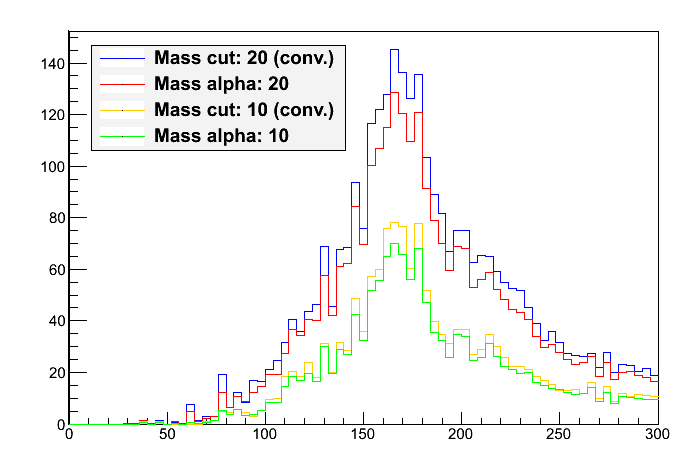
This finally allows a rough mass reconstruction with the cut of delta Mass <20GeV which is shown in the plot below (left): The red histogram shows combination with no jets in the others partition, whereas the green histogram represents combinations with one jet in the others partition. Apparently, the red histogramm shows a peak in the expected mass range (blue reconstruction), whereas the green does not show this – once again as expected. The plot shows decays without neutrinos (with >20GeV) only to avoid leptonic decays which makes the peak visible more clearly.
This gives confidence that the programs used for the previous analyses are working correctly and it is only due to the large number of partitions, that no signal was visible. Since now a signal peak is visible, one can compare different ways to put a cut on delta Mass – see the plot on the right. (The blue histogram here corresponds to the red histogram in the previous plot.) Two different conventional cuts were applied and two corresponding "smoothened cuts" (QJet-like) via assigning a weight of exp(-(deltaMass^2)/(alpha^2)). All weights are normalized per event to one, if any possibilities are found (in the conventional cutting method, this is why the conventional methods seem to have less entries). We can immediately see, that the smoothened cuts are have a quite similar distribution and not a notably better signal to backround ratio.
To simplify the previous efforts, in the next section, we only take a look at the jets that are a direct result of the t-tbar-decay. The plot to the right shows that these are only about 4-7 jets, which corresponds to 2-4 jets per produced top. Sometimes, jets may overlap, so that only three jets or two are visible, but this is not the usual case. The lower number of jets also decreases the number of possible partitions by several orders of magnitude. In average, there are now only about 10^3 possible partitions per t-tbar-decay (calculated by the formula above). This can still be reduced, as we know, that all of the jets should be included into either the top1 or the top2 partition, which leaves us with only 2^(n-1) partitions, i.e. less than 50 possible combinations in average.
This finally allows a rough mass reconstruction with the cut of delta Mass <20GeV which is shown in the plot below (left): The red histogram shows combination with no jets in the others partition, whereas the green histogram represents combinations with one jet in the others partition. Apparently, the red histogramm shows a peak in the expected mass range (blue reconstruction), whereas the green does not show this – once again as expected. The plot shows decays without neutrinos (with >20GeV) only to avoid leptonic decays which makes the peak visible more clearly.
This gives confidence that the programs used for the previous analyses are working correctly and it is only due to the large number of partitions, that no signal was visible. Since now a signal peak is visible, one can compare different ways to put a cut on delta Mass – see the plot on the right. (The blue histogram here corresponds to the red histogram in the previous plot.) Two different conventional cuts were applied and two corresponding "smoothened cuts" (QJet-like) via assigning a weight of exp(-(deltaMass^2)/(alpha^2)). All weights are normalized per event to one, if any possibilities are found (in the conventional cutting method, this is why the conventional methods seem to have less entries). We can immediately see, that the smoothened cuts are have a quite similar distribution and not a notably better signal to backround ratio.

 .
.
.
.
.
.
.
.
.
.
The following table shows the heuristically determined signal to background ratios:
.
.
.
.
.
.
.
.
.
.
The following table shows the heuristically determined signal to background ratios:
| cut type | cut at 20 GeV | alpha = 20 GeV | cut at 10 GeV | alpha = 10 GeV |
| signal/background | 1.7 | 1.8 | 2.0 | 2.0 |
The Positive Approach
 The positive approach is more based on the idea of conventional top reconstruction algorithms. These try to reconstruct for example by searching for the three jets with the highest combined p_T value or for jet combinations, that have the W-mass. As these approaches usually take relatively high cuts, they do not have too many possible combinations left. A cut could be regarded as the application of a Heaviside step function. A QJets-like approach here could be to smoothen this function. A good candidate might be 1/(1+e^(alpha*x)), where alpha is once again a rigidity variable. If the rigidity is very high (alpha*x >> 1), the function behaves like the heavyside function, if alpha is small (alpha*x << 1), all possibilities are taken into account.
This idea might make the QJets advantages (smoother distributions, additional variable "volatility") available to common top reconstructions.
-- GeorgJahn - 03 Apr 2012
The positive approach is more based on the idea of conventional top reconstruction algorithms. These try to reconstruct for example by searching for the three jets with the highest combined p_T value or for jet combinations, that have the W-mass. As these approaches usually take relatively high cuts, they do not have too many possible combinations left. A cut could be regarded as the application of a Heaviside step function. A QJets-like approach here could be to smoothen this function. A good candidate might be 1/(1+e^(alpha*x)), where alpha is once again a rigidity variable. If the rigidity is very high (alpha*x >> 1), the function behaves like the heavyside function, if alpha is small (alpha*x << 1), all possibilities are taken into account.
This idea might make the QJets advantages (smoother distributions, additional variable "volatility") available to common top reconstructions.
-- GeorgJahn - 03 Apr 2012 

| I | Attachment | Action | Size | Date | Who | Comment |
|---|---|---|---|---|---|---|
| |
comparison_cuts.png | manage | 12 K | 23 Apr 2012 - 13:02 | UnknownUser | A comparison on different delta Mass cuts |
| |
comparison_cuts_normalized.png | manage | 12 K | 24 Apr 2012 - 14:49 | UnknownUser | A comparison on different delta Mass cuts with bins normalized: one bin per event |
| |
heaviside.gif | manage | 3 K | 16 Apr 2012 - 15:55 | UnknownUser | heaviside like function |
| |
negap_dd_distribution.png | manage | 9 K | 16 Apr 2012 - 13:51 | UnknownUser | Direction Deviation Distribution |
| |
negap_deltamass_distribution.png | manage | 12 K | 16 Apr 2012 - 09:34 | UnknownUser | DeltaM distribution |
| |
negap_jetcount_distribution.png | manage | 12 K | 16 Apr 2012 - 12:44 | UnknownUser | Jet Count Distribution |
| |
negap_mass_distribution.png | manage | 12 K | 13 Apr 2012 - 16:23 | UnknownUser | Top Mass Distribution |
| |
negap_phi_distribution.png | manage | 12 K | 16 Apr 2012 - 10:00 | UnknownUser | phi distribution |
| |
negap_reconstruction_alpha_high.png | manage | 9 K | 17 Apr 2012 - 12:48 | UnknownUser | reconstruction alpha high |
| |
negap_reconstruction_alpha_higher.png | manage | 9 K | 17 Apr 2012 - 12:48 | UnknownUser | reconstruction alpha higher |
| |
negap_sumpt_distribution.png | manage | 13 K | 16 Apr 2012 - 12:21 | UnknownUser | pT-Sum distribution |
| |
onlytopjets_mass.png | manage | 9 K | 23 Apr 2012 - 09:40 | UnknownUser | Mass reconstruction from ttbar jets only |
| |
onlytopjets_number.png | manage | 9 K | 22 Apr 2012 - 16:28 | UnknownUser | Number of Jets >10 GeV directly correlated with ttbar production |
| |
partition_jet_count.png | manage | 9 K | 13 Apr 2012 - 16:07 | UnknownUser | Jet count in t-tbar-events at 14 GeV |
| |
to.png | manage | 9 K | 16 Apr 2012 - 15:53 | UnknownUser | Top Mass |
Edit | Attach | Print version | History: r10 < r9 < r8 < r7 | Backlinks | View wiki text | Edit wiki text | More topic actions
Topic revision: r10 - 24 Apr 2012, GeorgJahn
Ideas, requests, problems regarding Foswiki? Send feedback