Subpages

GroomedMassComparisons

GroomedMassComparisonsSinglePt (Gavin's version)

Robustness study

Rationale

The aim of this study is to establish the level of reliability of the prediction of our Monte Carlo simulation. Our studies into the identification of boosted objects using jet substructure rely on an accurate description of certain distributions (jet mass and splitting scales, either raw or after a certain amount of grooming).

Our results can be expected to be quite sensitive to the simulation of the parton shower. To get a feeling for the magnitude of this effect we compare two popular tools (Herwig 6.510 and Pythia6.4).

In the experimental environment there will moreover be some activity that is not directly related to the jet, but can affect its measurement: underlying event and pile-up. We cannot study the latter, but we'll probe the overall sensitivity for this type of activity by comparing different Pythia UE tunes. We compare the three tunes for which Gavin Salam produced samples:

- DW: Q^2 ordered shower with a reasonably realistic underlying event

- DWT: Q^2 ordered shower with an excessively noisy underlying event

- Perugia0: pt-ordered shower with what should be a reasonably
realistic underlying event.

Note that the DW and DWT use a different shower ordering than Perugia. It may be impossible to disentangle effects due to the parton shower modelling from those of the

Finally, the limitations in detecting all particles in the jet will change the distributions. Soft charged particles will be swept out of the jet by the magnetic field. Distributions will be smeared due to the limited calorimeter granularity.Thresholds are applied to deal with detector noise. It is impossible to study this without access to the full simulation (and the answer may not be the same for CMS and ATLAS or even for jets based on different objects (particle flow vs. calorimeter-only, towers vs. clusters). But, again, we hope that the comparison of the jets based on generator output and the detector objects returned by a tool developed by UW may help to understand what the typical magnitude for such effects is.

This comparison of different MC samples will establish the sensitivity or robustness of these observables to these effects (with the usual assumption that the differences between the models is a measure of the uncertainty). In the next year, a detailed comparison of data and MC will allow a detailed understanding of which tools and tunes work and which don't.

For other comparisons of different showers (and matched samples) in event-shape observables (which have some similarities to jet masses), see CMS-PAS-QCD-10-013.

Samples and analysis

The parton shower and UE study uses the samples generated by Gavin Salam (available under http://www.lpthe.jussieu.fr/~salam/projects/boost2010-events/pythia64/ and http://www.lpthe.jussieu.fr/~salam/projects/boost2010-events/herwig65/). The names for the different Pythia tunes are part of the file names. To keep things simple we focus on the di-jet sample and choose a single pT bin from 500-600 GeV (repeating the analysis in different pT bins gives similar answers).The cross-sections for the four samples (0.0443 nb, 0.0442 nb, 0.0451 nb and 0.0421 nb for Pythia DW, DWT, Perugia0 and Herwig, respectively) agree within 7% (difference between the highest and the lowest value). In the analysis we concentrate on the shape and normalize all distributions to unit area.

Corresponding event samples with multiple interactions (UE) turned off can be useful for distinguishing which effects come from the shower and which ones from the UE. They're available (in just one pt bin) from http://www.lpthe.jussieu.fr/~salam/projects/boost2010-events/noUE/

For the detector study we use the Seattle samples. In particular, we use four files:

http://tev4.phys.washington.edu/TeraScale/dijet.pt0500-0600.01.UW.gz

http://tev4.phys.washington.edu/TeraScale/dijet.pt0500-0600.01.UW.detector

http://tev4.phys.washington.edu/TeraScale/ttbar.pt0500-0600.01.UW.gz

http://tev4.phys.washington.edu/TeraScale/ttbar.pt0500-0600.01.UW.detector

For each of the samples jet are reconstructed using the anti-kT algorithm with R=1. For each of the jets kT is rerun on the constituents and the splitting scales are obtained. This is implemented as a simple standalone programme linking to FastJet and ROOT. No grooming is implemented (yet).

Results

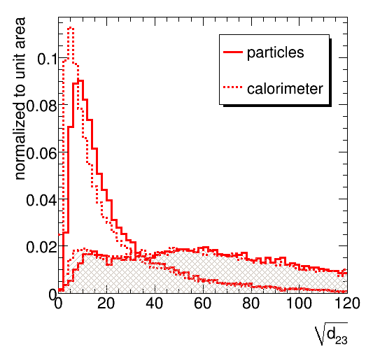
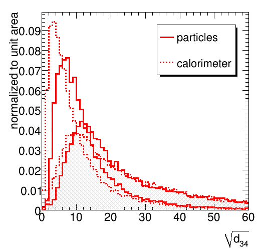
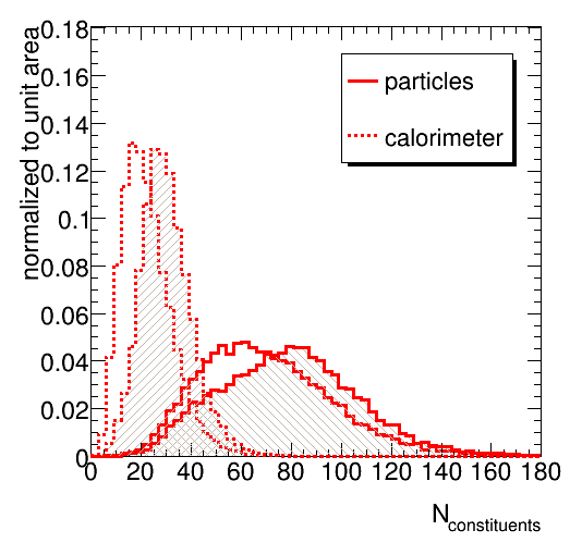
The jet mass distributions for four di-jets samples with 500 < pT < 600 GeV are shown below. The difference between Pythia and Herwig mentioned by several people during the workshop is indeed confirmed. The Herwig jet mass spectrum is significantly harder. The three tunes of Pythia show less variation. The larger (excessive) UE activity in DTW with respect to DW indeed leads to a softer distribution. Perugia0 leads to a significantly softer spectrum, which could be due to differences in the UE tune or due the different shower ordering used.

Many of our analyses use this observable to distinguish mono-jets stemming from the decay of a heavy new particle from the QCD background jets stemming from a single quark or gluon. The result will be strongly affected by the choice of MC tool. As an example, consider the fraction of QCD di-jet events in a mass window between 166 and 207 GeV (values inspired by a desire to contain the top signal). For DW, DTW, Perugia0 and Herwig one would integrate, respectively, 6.6 %, 7.3 %, 4.8 % and 8.6 % of the events in the 500-600 GeV sample. The choice of MC can thus leads to nearly a factor 2 difference in our performance estimate.This result, although not unexpected, clearly shows the need for detailed studies on data. It seems likely that MC tuning will have to take into account jet substructure explicitly.

Four other observables reflecting the jet substructure are shown below (the first, second and third splitting scale of the kT cluster sequence on the jet constituents and the number of constituents. Note that the d12, d23 and d34 are obtained with R=0.3. This causes the plotted sqrt(d_ij) to be larger be factor sqrt(3.333) than you might expect. The R=1 distributions is actually not exactly obtained by merely scaling, so the plots will be repeated with a uniform definition of R in both jet algorithms. Thanks to Bertrand for spotting this.). We again choose a window on each of these distribution that selects 60 % of a top signal in the Herwig sample, choosing the window boundaries so they remove 20 % of the signal on both sides. This procedure selects the following fractions of di-jet events. For d12: 17% (DW), 17% (DWT), 11% (Perugia) and 16 % (Herwig). For d23: 23 % (DW), 22 % (DWT), 17 % (Perugia) and 25 % (Herwig). For d34: 7.7 % (DW), 7.7% (DWT), 6.9 % (Perugia) and 7.5 % (Herwig). The same pattern is thus observed in the three observables: reasonable agreement between the Q^2 ordered showers in Pythia and Herwig, while the Perugia tune clearly stands out.

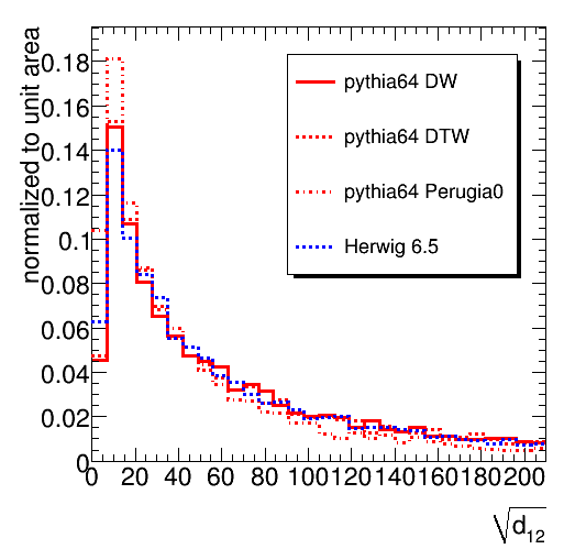
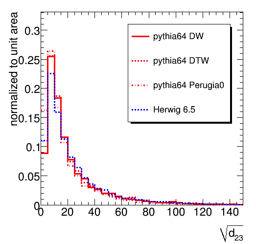
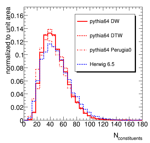The number of constituents differ significantly between the different tools and tunes.

One would hope the prediction for the splitting scales (reflecting a relatively hard event in the shower development) is less sensitive to at least the uncertainty in the Underlying Event than the jet mass (where something soft on the jet periphery can ruin everything). This is confirmed by the relatively small difference between the d12, d23 and d34 distributions returned by Pythia DW and DWT and Herwig. The results from the Perugia0 sample, however, cannot be made to fit in this simple picture. Feedback from jet and generator experts is welcome.

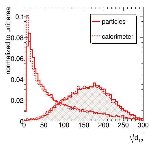
The next step is to compare particle jets to detector jets. The limited detector granularity and the presence of a 1 GeV threshold for cells are simulated by a tool provided by UW (to be replaced by Peter Loch's more sophisticated treatment when that arrives). The jet mass is found to be quite sensitive the detector effects. The peaks of the distributions for both a top signal and the QCD jet background are shifted down by 10 GeV (some of this is expected to be due to the 1 GeV threshold, some due to merging of several particles in massless calorimeter clusters). The signal peak is slightly broader and the mass window to contain 60% of the signal must be opened accordingly. Unfortunately, the high mass tail of the background is not affected very much. A more pronounced tail towards low mass develops in the signal sample. The fraction of QCD jets in the mass window increases from 8.3 % to 9.4 %.

The prediction for the splitting scales, shown in the figures below, is more robust. For the signal, the first splitting scale hardly varies at all. As a rule of thumb, the softer the splitting, the more it is affected. We see significant differences in the range up to several tens of GeV in all distributrions, but beyond 20-30 GeV the agreement is quite satisfactory.

Conclusions

The jet mass is found to be quite sensitive to the parton shower model and detector effects and, to a lesser extent, to the underlying event description in the Monte Carlo. Variation of the MC description in a range that (more than) spans the uncertainty leads to significant effects. An estimate of the probably to mistag a QCD jet as a boosted decay of a heavy (exotic) particle can vary by up to nearly a factor 2. It is therefore suggested that future studies are performed on a well-defined benchmark set to allow comparison on an equal footing.

The reliability of MC predictions of jet substructure must be addressed urgently, as the LHC is entering the boosted regime. In the next year, the comparison with LHC data will allow for a much better understanding of the performance of the Monte Carlo tools. To take full benefit, observables that probe jet substructure must be taken into account explicitly in the tuning of MC tools on LHC data.

Observables that measure relatively hard events in the shower development, like the splitting scales used in many taggers, can be a more robust probe of jet substructure than the jet mass. This is particularly true if the selection avoids the region of low scales (below 20-30 GeV), a condition that can easily be met in practice.

Performance studies: Definitions

Performance Study: Definitions (cf. E-Mail from James from July 13th)

Samples

Herwig 6.510 and Jimmy 4.31

Background:

http://www.lpthe.jussieu.fr/~salam/projects/boost2010-events/herwig65

herwig65-lhc7-dijets-pt0200-0300.UW.gz
...
herwig65-lhc7-dijets-pt0700-0800.UW.gz


and for signal:

herwig65-lhc7-ttbar2hadrons-pt0200-0300.UW.gz

herwig65-lhc7-ttbar2hadrons-pt0700-0800.UW.gz

Pythia 6.421

Samples generated with Pythia 6.421 can be found at

http://www.lpthe.jussieu.fr/~salam/projects/boost2010-events/pythia64

Names are as for Herwig, except that the pythia tune is also specified in the filename, e.g.:

pythia64-tuneDW-lhc7-dijets-pt0300-0400.UW.gz

3 tunes are available:

• DW: this is a widely used tune of the the virtuality-ordered shower (Q2), with an underlying event that's about right (at least in terms of energy flow) for LHC7.
• DWT: identical to DW at Tevatron, but with different energy scaling of the UE parameters; it should be about 30% more active than DW at 7 TeV (roughly equivalent to about 1 additional pileup event).
• Perugia0: this is a modern tune of Pythia's (6.421) pT-ordered shower; the UE should also be about right here?

By comparing the Pythia and Herwig results (different showers, different UEs) we should obtain one measure of the extent to which efficiency and fake-rate results are robust.

Tagging Optimization

As for the validation plots, find the jets with antikt R=1.0 first. As for validation, use all particles with abs(eta) < 5 except neutrinos and muons. In the further study, only consider jets with p_T > 200. Consider only at most 2 jets per event, i.e., exclude the p_T-third, p_T-fourth jet in an event, even if it has p_T > 200.

Run the different taggers on the constituents of the jets found. If citing a jet p_T, this should always be the p_T of the antikt-jet initially found.

Run the tagger on all samples above and try to find optimal parameter values for the tagging. As result, give:

• for each of the p_T samples above, the number of found antikt "initial" jets with p_T > 200
• the tagging rate for the signal and background sample if optimizing for an overall efficiency of 0.1, 0.35, 0.5 and 0.9. Overall efficiency is defined as the number of tagged jets divided by the number of initial antikt jets with p_T > 200. Sum all samples. Use pure jet numbers as they are in the sample; do not apply any weight.
• distribution of variables used for the tagging, such as number of subjets, estimated top mass, W mass, ... for signal and background. Do this also seperately for the different p_T samples in order to see a possible p_T dependency of these variables. A 2D-plot variables versus jet p_could be helpful.

Taggers -> Groups mapping

• John's Hopkins Tagger - Minho
• Thaler Wang tagger - James
• ATLAS 09 style tagger (spitting scales) -Bertrand
• CMS Style tagger (although similar to JH) - Karlsruhe (Jeannine, Jochen, Jaakob)
• Almeida et al. style (planar flow) - Gilad and collaborators?
• Pruning style tagger - Chris?
• Chekanov-Proudfoot -
• CM tagger - Gavin?
• (Plehn et al tagger - to be decided if included at all)

Performance Study: Results

KIT group

We found overall 111911 considered initial jets (antikt 1.0, p_T > 200) in signal, 114758 in the background sample. Parton p_T is the p_T of matched top to an inital jet. Here deltaR < 0.8 between top and intial jet was used for matching. After this we have 111129 signal and 113618 background events. The combined p_T spectrum for these jets can be seen here:

The algorithm attempts to decompose the jet into 3 or four hard subjets. The number of actually found subjets can be seen here:

After finding the subjets, cuts are placed on the mass of the original jet and m_min, defined as the minimum mass calculating all possible pairings of the three pt-hardest subjets. While the jet mass is defined for all jets, m_min is only defined for jets with at least 3 subjets.

Scanning through possible cut values for m_min and m_jet and taking the cuts with the smallest mistag rate for a given efficiency yields the following curve:

The working points were set to 10%, 35%, 50% and 90% efficiency. The 90% efficiency is not reached because a considerable fraction of signal jets has only 2 hard subjets. This yields to a maximum reachable efficiency of about 60% for the considered sample. The mistag rates at the remaining working points are:

efficiency [%]	mistag rate [%]	cut on m_min > ... GeV/c^2	cut on m_jet in interval
10.3	0.27	75	[160, 185]
34.5	1.5	67.5	[160, 230]
50.6	5.4	42.5	[160, 285]

For these results, no explicit limit on the minimum widths of the mass window was set. Following James' suggestion to put a lower limit for the mass cuts of 40 Gev changes the first row in the table which then has a mistag of 0.33% with cuts of m_min > 75 and m_jet in [140, 185].

As proposed in the ongoing email discussion. We plotted for the overall optimisation the mistag rate vs. tag rate for each p_T sample. Further we present the same result optimising for each p_T sample individually.One sees that the higher the p_t samples the better the ROC-curves. For p_T sample > 500 GeV/c the differences in the ROC-curve are small.
Optimising for each sample individually does not yield better ROC-curve (higher efficiency by same mistag rate). However one obtains the same curve, meaning: going towards higher efficiencies yields higher mistag rates.

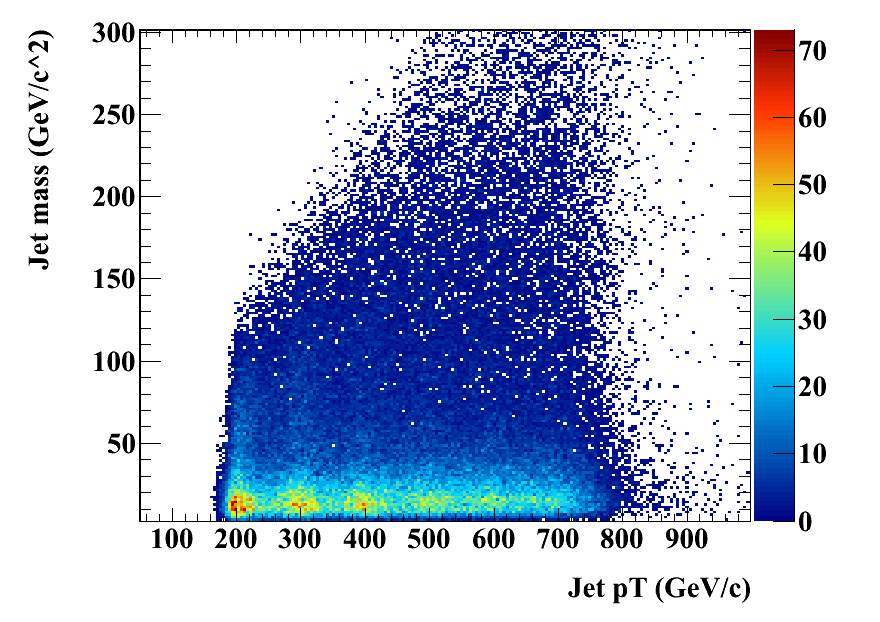
The p_T dependence of the variables used for tagging, m_min and m_jet. The structure at p_T around 200-300 Gev/c at a jet mass of below 100 Gev indicates that these jets fail to collect all the top quark decay products but rather only collect the W (or a combination of other two quarks). Note that on the right hand plot, only those jets with >= 3 subjets are used because only for them, M_min is well-defined. Therefore, there is no corresponding structure in the right hand plot. Apart from this structure, there is little pt-dependence of m_jet and m_min.

The same 2D plots for background:

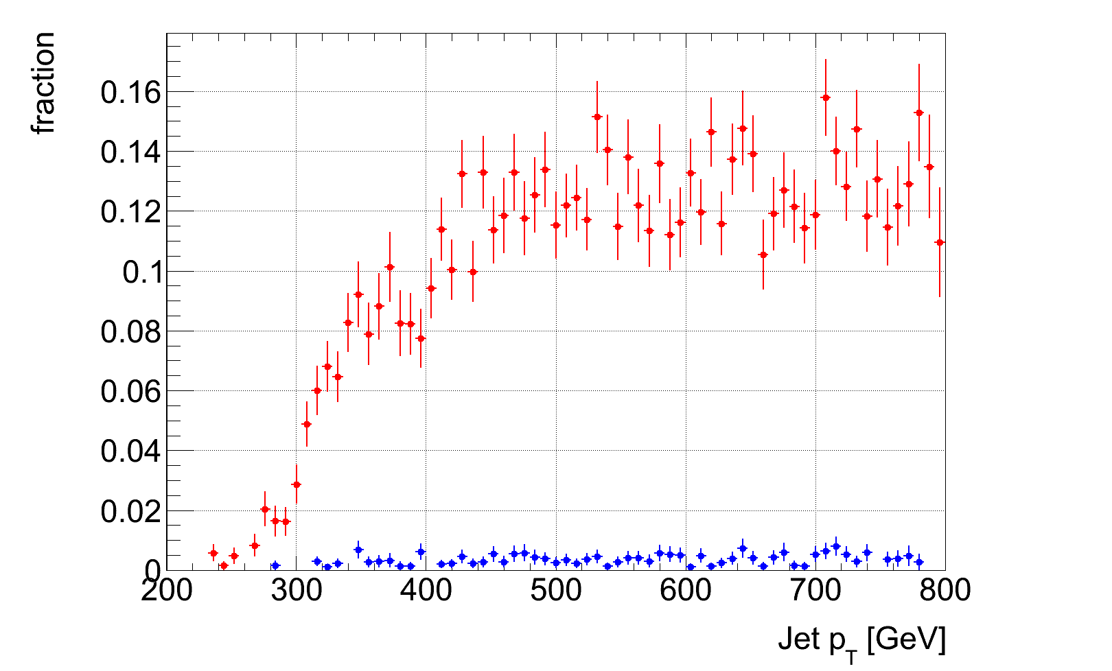
For the selected working points 0.1, 0.35 and 0.5 we plotted the tag rate and mistag rate over the whole jet p_T as well as over the parton p_T range. Parton p_T is defined as mentioned above, DeltaR < 0.8 between initial top and jet. In the plots we just show the p_T range 200-800 GeV/c leaving out p_T > 800 due to low statistics as can be seen in the N over p_T plot.

For the overall efficiency points 0.35 and 0.5 the curves seem to saturate for p_T > 500 GeV/c.

And for each working point we plotted efficiency and mistag rate over jet p_T and parton p_T. In order to better see the mistag rate we scaled the background with factor of 5.

Yale

Initial jets (antikt with R = 1.0, p_T > 200) are 111911 for signal, 114758 for the background sample.

Each anti-kT jet is individually reclustered by Cambridge/Aachen algorithm with R = 1.5 (an arbitrarily big size to ensure that all constituents of anti-kT jet are captured). The resulting jet is merely same as the initial anti-kT jet except the different clustering sequence. Next each jet is declustered to look for subjets according to [arXiv:0806.0848]. This is done by reversing each step in the Cambridge/Aachen clustering, iteratively separating each jet into two objects. The softer of the two objects is thrown out if its pT divided by the full jet pT is less than a parameter delta_p, and declustering continues on the harder object.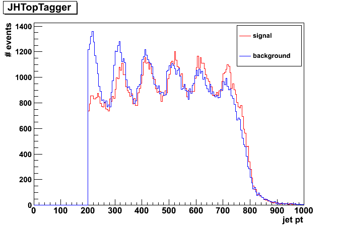

Left: jet pt distribution, Right: jet mass of each pt bin (to get some idea of how likely top constituents merge with varying pt).

In JH top tagger style, the hardness of the declustered objects is defined by a parameter delta_p that measures a relative pT with respect to full jet pT. Therefore, the number of hard objects within each jet is sensitive to this parameter. In order for background to look like a decayed top quark, a hard parton must at least undergo two branchings at somewhat large angles and energy sharings, which is relatvely rare. This is what we see in the above plot, or the fraction of jets (of dijet background) that have at least two branchings rapidly drops as delta_p increases. We have divided the number of maybe-top jets (, or N subjets >2) by min(2, pt > 200) (Recall that we have selected only first one or two hardest initial anti-kT jets that passed pT cut and applied top tagger on these selected jets).

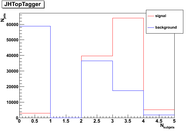
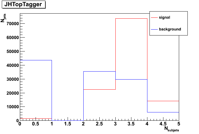Left: number of subjets for delta_p = 0.18, Middle: number of subjets for delta_p = 0.08, Right: number of subjets for delta_p = 0.04. (these three choices correspond to the three working points, 10, 35, 50%).

Optimization: JH Top Tagger has delta_p, delta_r variables at declustering. Since pT of all signal and background samples is well smaller than 1 TeV-scale, I have fixed delta_r to be 0.19 as default. I have optimized over four variables, or delta_p, mW, mtop, cos_theta_h where mW and mtop are reconstructed invariant masses. Range of scanned variables (note that I have fixed the lower value of mass window to ease optimization):

delta_p	delta_r	mtop	mW	cos_theta_h
0.001-0.2	0.19	[140,180-280]	[60,80-120]	[0, 0.6-1.]

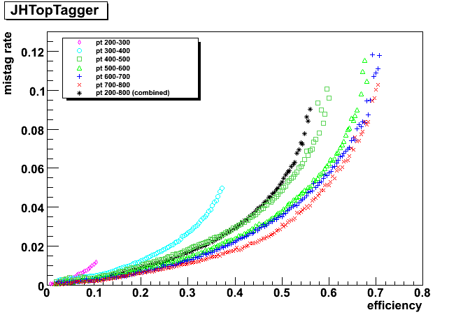As you can see in the plot (black color), It seems to be very hard to get overall efficiency higher than around 60% for all samples.

Working Points:

efficiency [%]	mistag rate [%]	delta_p	delta_r	mtop	mW	cos_theta_h
10.4	0.36	0.18	0.19	[140, 196]	[60, 88]	< 0.64
35.2	2.2	0.08	0.19	[140, 216]	[60, 102]	< 0.74
50.0	5.3	0.04	0.19	[140, 262]	[60, 120]	< 0.86

Top tag rate vs jet pt for two working points, 10% , 35%and 50%.

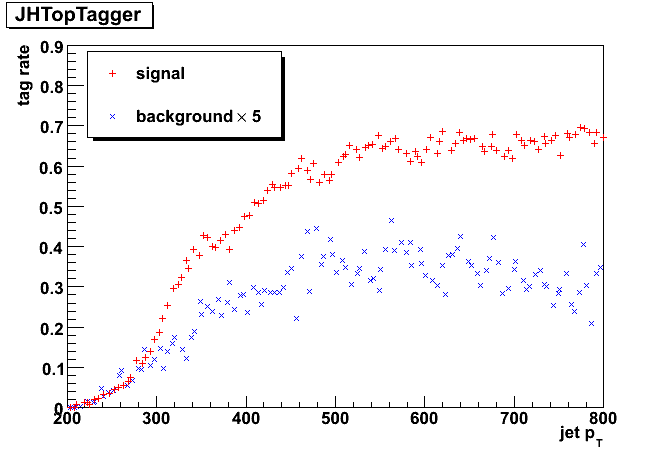Left: overall eff. of 10%, Middle: overall eff. of 35%, Right: overall eff. of 50%.

*Some detail study of efficiency = 35% case.

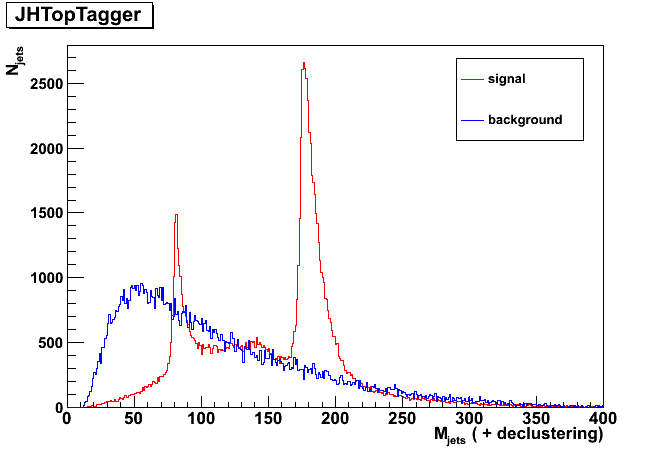
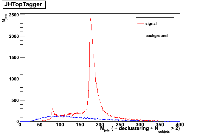The first plot is just jet mass. the second plot is jet mass after declustering procedure implemented in JH top tagger, and the last plot is jet mass of top candidates (only required the number of subjets greater than 2).

Eff.=35%	signal	background
initial anti-kT jets (reclustered by CA)	111911	114758
+ N subjets > 2	69163	19367
+ pass Top mass	49429	5283
+ pass W mass	46436	4165
+ pass helicity angle	39396	2553

Seattle group: pruning

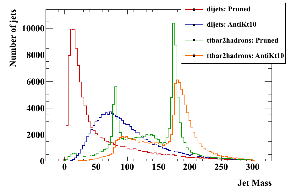
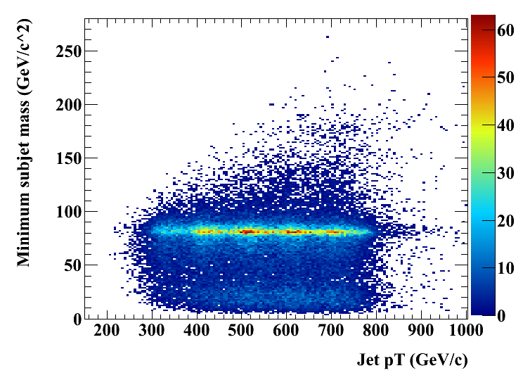
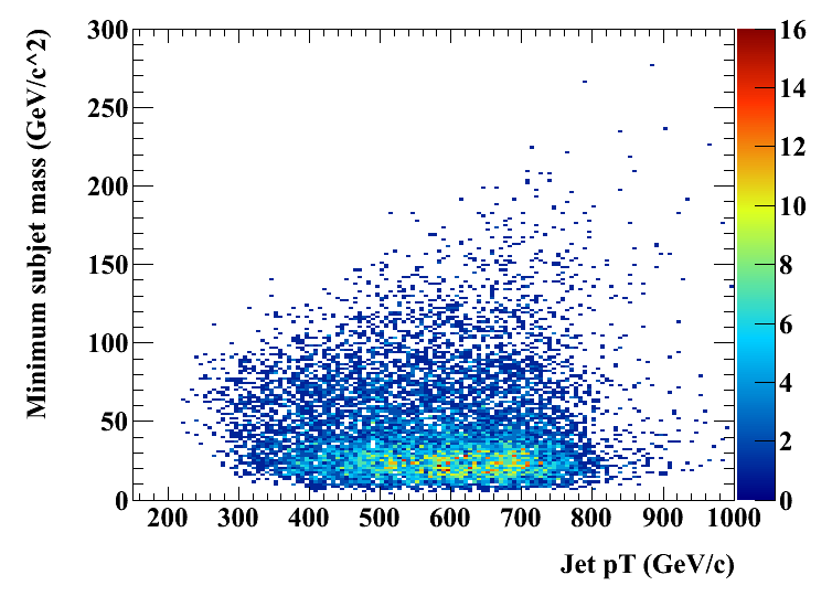
The initial jets should be the same as the other analyses; here is the pT spectrum at a check: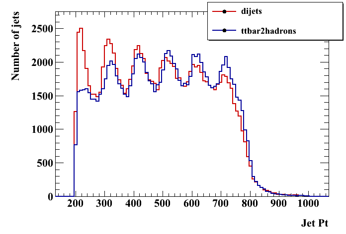

Pruning operates on each jet to remove extra radiation, with the goal of narrowing the signal mass distribution and lowering the background mass distribution. So the relevant variables are just the jet and subjet masses. Here are these distributions for signal and background, pruned and unpruned. The pruned plots use the "standard" values suggested in the original reference, z_cut = 0.1, D_cut = 0.5*(2m/pT). Two subjet mass plots are shown. In the first, the heavier subjet is assumed to be the W (this method was used in the original pruning papers). In the second, a form of the "minimum mass" selector as in the CMS tagger is used -- the final jet is unclustered to three subjets, and the pair with the minimum mass is merged. This does slightly better at reducing the background. In the subjet mass plots, the jet mass is required to be greater than 150 GeV.

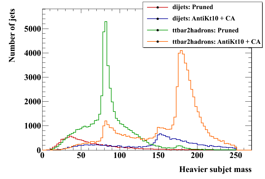
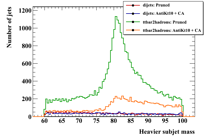
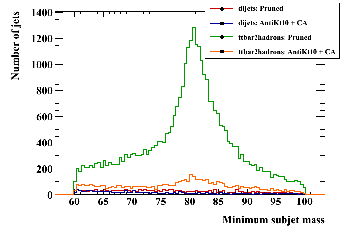To explore the efficiency space, the following parameters are varied:

z_cut	D_cut / (2m/pT)	m_W window	m_top window
[0, 0.2]	[0.1, 0.85]	[20, 120]	[40, 140]

The W and top mass windows are centered on the mass peak, found by fitting the signal curve (see arXiv:0912.0033 for details). The windows have lower bounds of 60 GeV and 140 GeV respectively. The efficiency scatter plot is shown below.

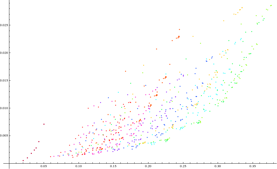Each color is a different value of z_cut, and the groups for each color represent the different mass window sizes (the W and top windows are varied together). Picking out some specific points, we have:

efficiency [%]	mistag rate [%]	z_cut	D_cut	mtop	mW
9.8	0.13	0.2	0.2	[150.6, 190.6]	[68.3, 88.3]
32.5	1.42	0.075	0.4	[140, 212.1]	[60, 118.6]

40% appears to be about the maximum efficiency achievable, given the lower bounds on the mass cuts.

If we allow the mass windows to be smaller, I get the following efficiency curve:

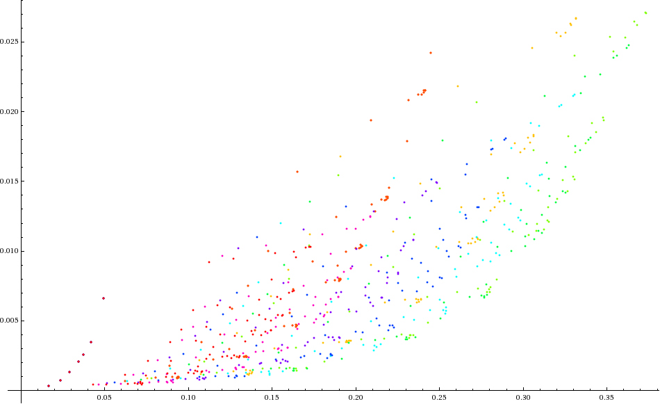At the 10% efficiency point, we can now achieve {9.8%, 0.082%} :

efficiency [%]	mistag rate [%]	z_cut	D_cut	mtop	mW
9.1	0.058	0.175	0.4	[166.9, 181.6]	[74.3, 87.7]
9.8	0.082	0.15	0.55	[67.5, 183.0]	[74.1, 88.8]
32.5	1.42	0.075	0.4	[140, 212.1]	[60, 118.6]

Now, let's look at the pT dependence. Here are signal and background plots for jet and (minimum) subjet mass vs. pT:

McGill

Unlike usual taggers, no grooming procedure is attempted here. Apart from the jet mass (which is taken straight from the inital jet), the different observables that are used are reconstructed by feeding the jet constituents to the kT algorithm and undoing the few last stages of the clustering. The observables are :

• the jet mass
• the W candidate mass : invariant mass of the subjet pair with lowest mass (when the jet is forced to split into 3 subjets)
• z_cut_12 = d_cut_12/(d_cut_12 + jet mass^2)
• z_cut_23 = d_cut_23/(d_cut_23 + jet mass_2^2)
• z_cut_34 = d_cut_34/(d_cut_34 + jet mass_3^2)

For the last three variables, d_cut is the kT splitting scale. This definition of z_cut variables is such that correlations with respect to the jet mass is (at first order) minimal.

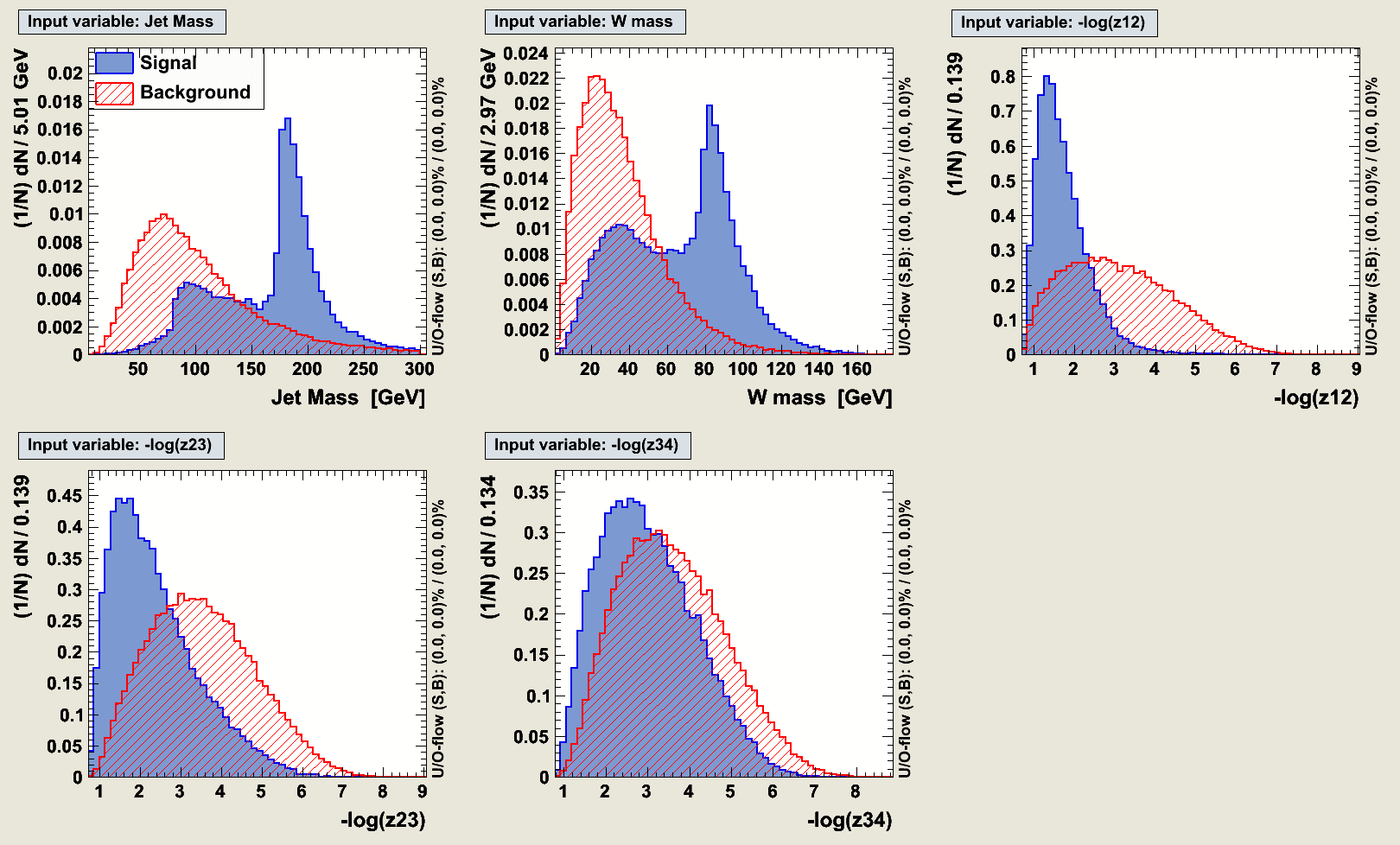The optimisation has been done via a projective likelihood. TMVA analysis package was used for the construction of the likelihood ratio. A linear decorrelation transformation on the input variables was also applied; it doesn't increase drastically the performance of the classifier but it still does a little bit. For practical purposes, only jets with jet mass < 300 GeV are considered.

ROC curves:

plain lines = optimised over all samples, applied on the specific (pT) samples.

dashed lines = optimised and applied on the specific samples.

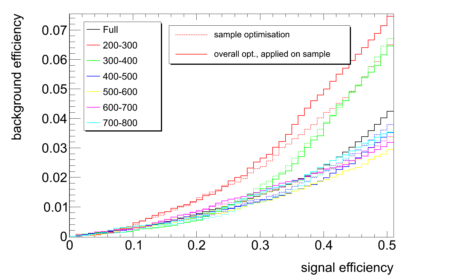(The right plot is a close up view of the the left one).

The interpretation of those curves needs to be done with care as this is a bit misleading since for low pT samples (i.e. 200-300 notably), we end up optimising for boosted W's (qq') or bq, bq' (which = most of the signal). Those curves relate to top-tagging for the highest pt samples where most of our signal = boosted tops.

Efficiency matrix, mistag rate as a function of signal efficiency and pT sample:

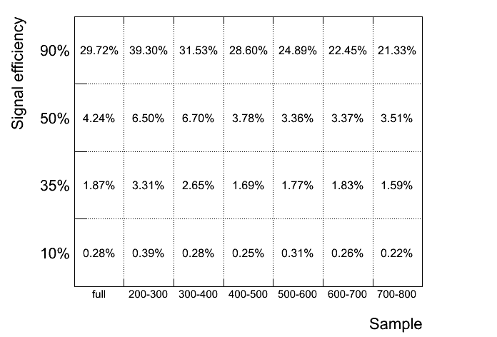As an alternative, one can train the classifier on the 700-800 pT sample and apply the selection on the other samples. The following ROC curves are obtained (same color scheme as above) and efficiency matrix:

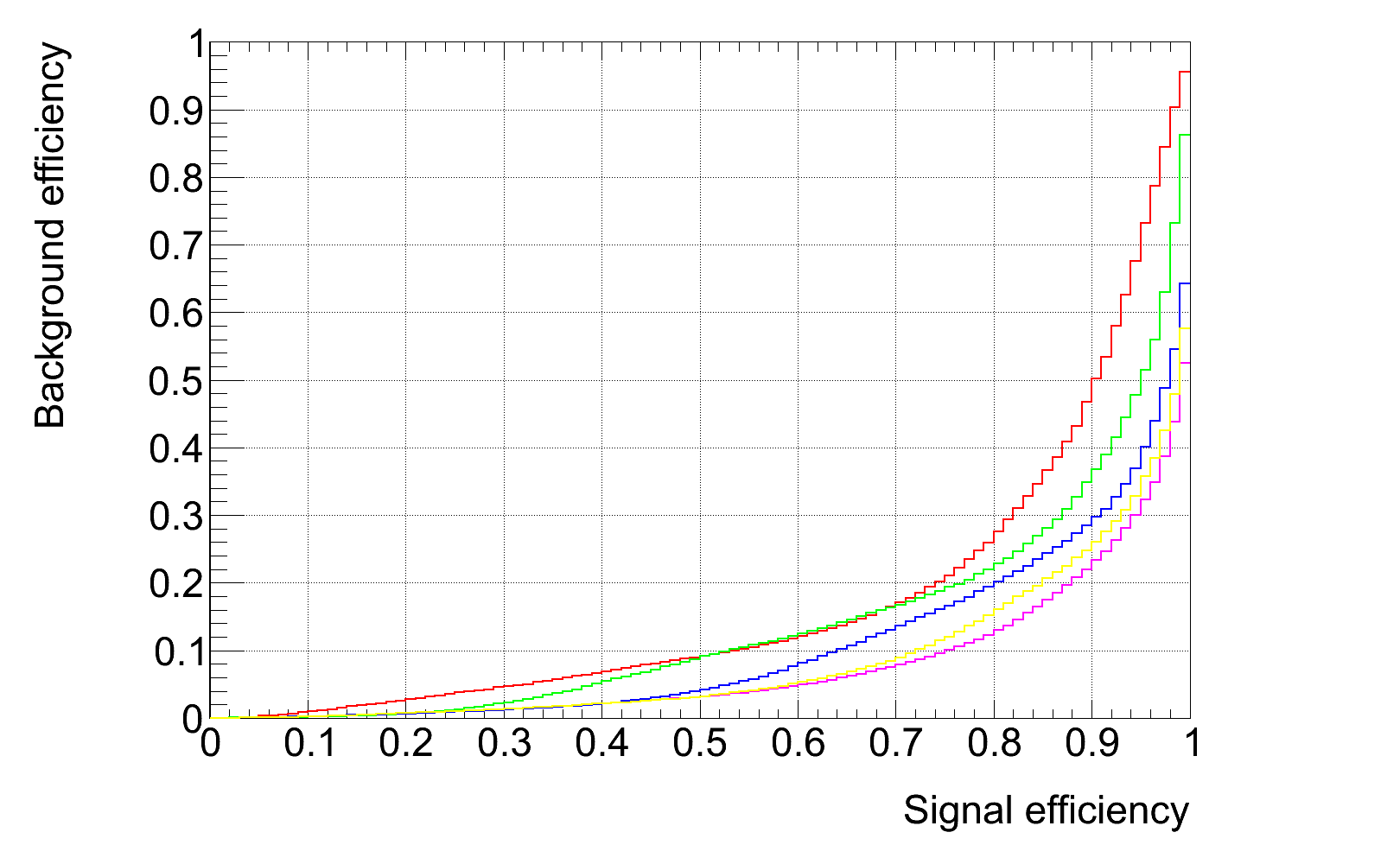
To avoid optimizing for boosted 2 body decays (e.g. bootsed W's), a 120 GeV cut on the jet mass in enforced on all tagged jets, in addition of the cut on the classifier (projective likelihood) output. Resulting ROC curves and efficiencies vs Jet pT shown below.

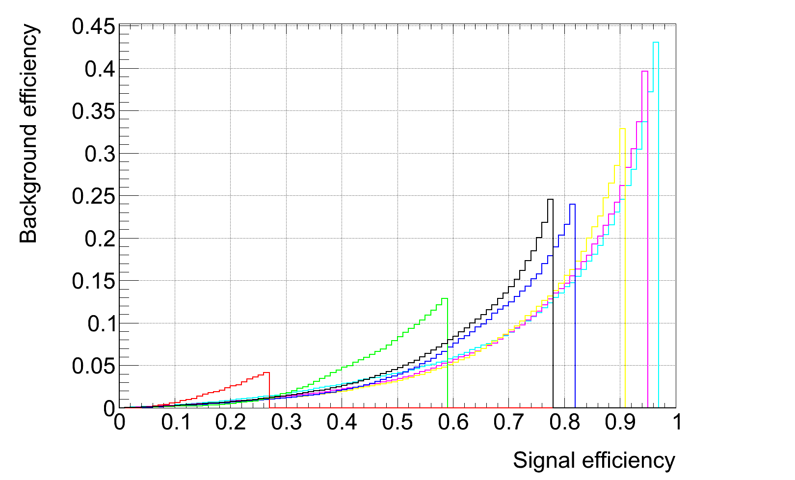10% signal efficiency working point

35% signal efficiency working point

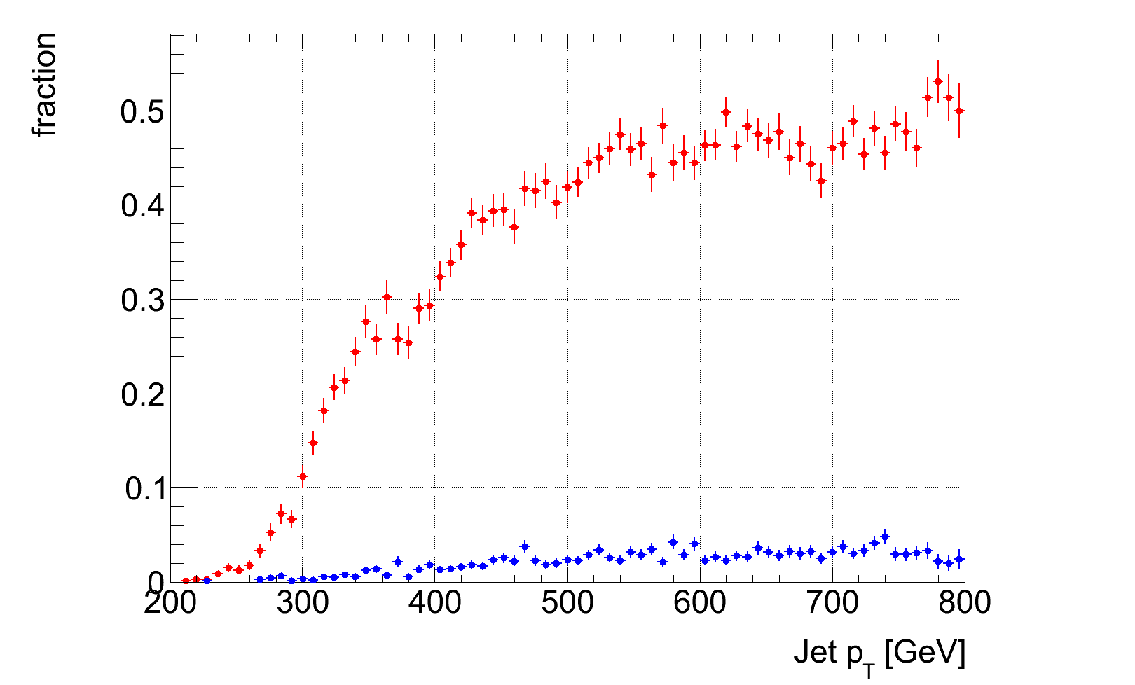50% signal efficiency working point

Oxford

Another candidate algorithm is the Thaler and Wang algorithm. On which the ATLAS algorithm evaluated by McGill is based. It only considers information from the first and second splitting of the exclusive k_T algorithm as appllied to the constituents of Anti-KT R=1.0 jets. The variables available are:

• the jet mass
• the W candidate mass : invariant mass of the subjet pair with lowest mass (when the jet is forced to split into 3 subjets)
• z_cell = min(E_1,E_2)/(E_1+E_2)) where E_1 and E_2 are the energies of the 2 subjest from forcing the initial jet to split into 2 subjets.

These variables are shown for the combination of all variables below:

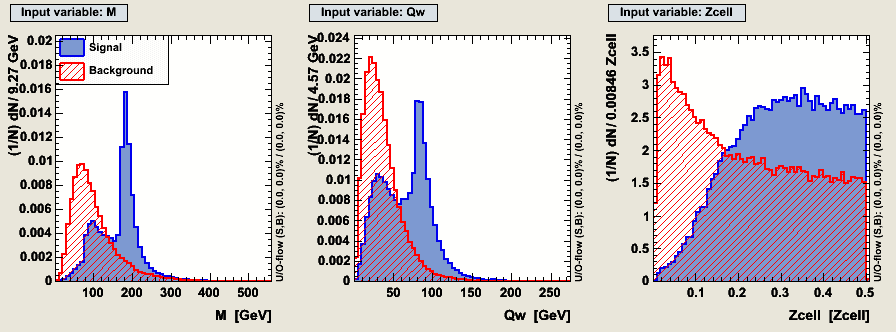Optimisation of cuts was performed using TMVA-v4.0.3. Cuts were optimised via both a Genetic Algorithm and a Monte Carlo method.

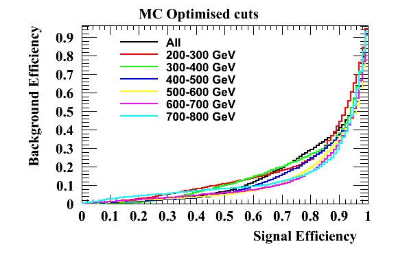
Similar caveats apply to the efficiencies as for the McGill selection.

An interesting feature is that here the optimisation over all %$p_T$%s does not perform so well as the individual %$p_T$% ranges in the mid efficiency range.

Numbers for the working points (MC optimisation)

Signal Eff	Background Eff (all)	Cuts (all)	Background Eff (400-500)	Cuts (400-500)	Background (700-800)	Cuts (500-700)
90%	40.8 %	M>84.5, Qw>8.6, Z_cell>0.102	35.8%	92 < M, 3.3 < Qw, 0.104 < Zcell	29.9%	141 < M, 33 < Qw, 0.0406 < Zcell
50%	6.73%	M>169, Qw>60, Z_cell>0.117	4.45%	162 < M , 63 < Qw, 0.0366 < Zcell	6.61%	175 < M, 75 < Qw , 0.225 < Zcell
35%
10%	1.09%	M>164, Qw>80, Z_cell>0.396	0.696%	156 < M , 76 < Qw , 0.396 < Zcell	1.40%	178 < M, 83 < Qw,0.427< Zcell

Numbers for the working points (GA optimisation)

Signal Eff	Background Eff (all)	Cuts (all)	Background Eff (400-500)	Cuts (400-500)	Background (700-800)	Cuts (500-700)
90%	40.7 %	541> M>82.9, Qw>4.5, 0.539 > Z_cell>0.110	35.7%	92 < M < 460 , 3. < Qw , 0.102 < Zcell < 0.514	29.9%	139 < M < 592 29 < Qw, 0.0613851 < Zcell <= 0.560716
50%	7.01%	441> M>169, Qw>57, 0.511 > Z_cell>0.129	4.3%	166< M < 274, 59 < Qw , 0.0121 < Zcell < 0.499	7.28%	151 < M < 398 , 75 < Qw, 0.232 < Zcell <= 0.704
35%
10%	0.631%	224 > M>172, Qw>68, 0.586 %gt; Z_cell>0.398	0.581%	72 < M <219, 87 < Qw , 0.294< Zcell 0.588	1.12%	151 < M < 201 ,72 < Qw, 0.397656 < Zcell <= 0.586

Efficiency at 3 different working points as a function of P_T jet (blue is background, red signal) are below:

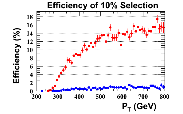
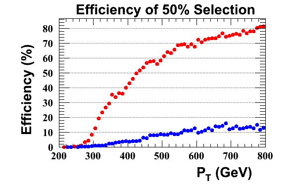
The following plots and tables are an update after adding in an m_jet > 120 GeV cut as a prerequisite on the tagger to avoid optimising for non-top jets. In all cases optimisation has been preformed across the full P_T range.

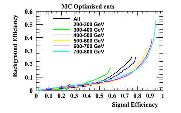
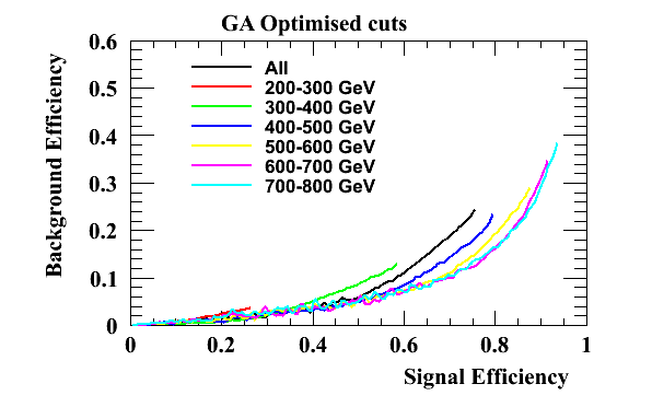The GA optimsied working points are used here:

Signal Eff	Background Eff (all)	Cuts (all)
50%	6.2%	582> M>155, Qw>42, 0.511 > Z_cell>0.110
35%	3%	267> M>165; Qw>69, 0.588 > Z_cell>0.215
10%	0.4%	223 > M>120, Qw>80, 0.298 > Z_cell>0.129

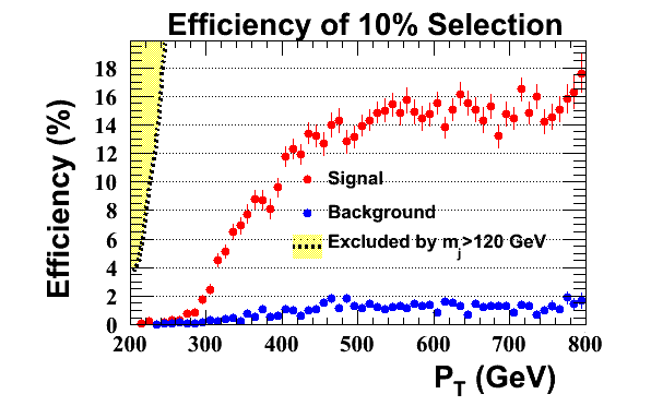
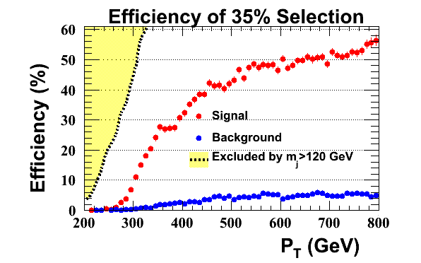
Davis group

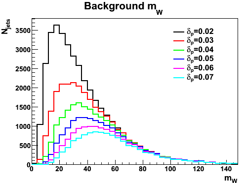
Here are some additional studies of the CMSTopTagger to add to the KIT group's results. Systematic studies of algorithm variables such as the momentum fraction parameter delta_p were performed. Pt binned samples are combined without weighting.

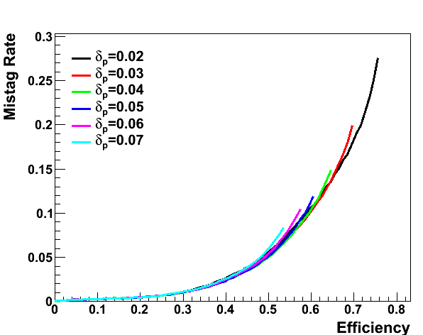
Validation Plot: Definition

Samples

• ttbar: http://tev4.phys.washington.edu/TeraScale/ttbar.pt1000-1100.01.UW.gz
• dijet: http://tev4.phys.washington.edu/TeraScale/dijet.pt0900-1000.01.UW.gz
• Higgs: http://tev4.phys.washington.edu/TeraScale/ZH.pt1000-1100.01.UW.gz

To cluster jets, use all stable particles with abs(eta) < 5 except neutrinos and muons.

Examples of how to read in the UW format are given in Gavin's tutorial

Top Tagging

Use antikt R = 1.0 as initial jet algorithm and use a cut of p_T > 400 on these.

On the constituents of the antikt jets, run the Cambridge/Aachen with R=1.0 as "initial" algorithm. Then apply different substructure search algorithm.

• John's Hopkins tagger. Use http://www.lpthe.jussieu.fr/~salam/fastjet/tools-code/JHTopTagger.hh . Use the default parameters given in the code: delta_p = 0.1, delta_r = 0.19 and mW = 81.0. For further study / plots, only use jets for which >=3 subjets have been found (i.e.,the method maybe_top() returns true).
• CM tagger. Use http://www.lpthe.jussieu.fr/~salam/fastjet/tools-code/CMTopTagger.hh with parameters zmin=0.1 and mass_max = 0.0. For further study / plots, only use jets for which >= 3 subjets have been found (i.e., the method maybe_top() returns true).
• Jet Pruning. Use http://www.phys.washington.edu/groups/lhcti/pruning/FastJetPlugin/FastPrune-0.4.0.tar.gz. Use the default parameters zcut = 0.1 and rcut_factor = 0.5. Fr further study / plots, only use jets for which actually two subjets have been found (which are required to define the W mass).

For each jet, plot:

• jet mass of the initial jet
• top mass as defined by the respective tagging algorithm
• W mass as defined by the respective tagging algorithm

For each of these nine combinations of algorithm and variable, draw signal and background into one plot for comparison.

Higgs

Use antikt R=1.2 as initial jet algo and use a cut of p_T > 200 on these.

On the constituents of the antikt jets, run the Higgs tagger (http://arxiv.org/abs/0802.2470), available in fastjet at example/fastjet_boosted_higgs.cc

For each jet, plot:

• jet mass of the initial jet
• jet mass after the Higgs tagger has run

Validation Plot: Results

Put your plots here.

KIT group

Top study

47,072 jets in the signal ttbar sample and 52,201 jets in the background dijet sample passed the cuts on the antikt jets.

Cambridge/Aachen 1.0 jets: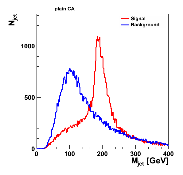

CM top tagger (46,805 jets in the signal sample, 51,602 jets in the background sample):

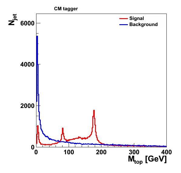
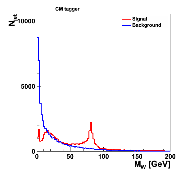
JH top tagger (19,797 jets in the signal sample, 5,266 in the background sample):

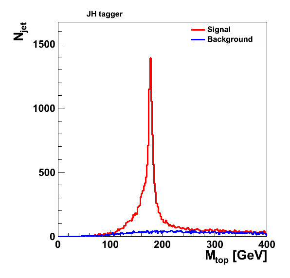
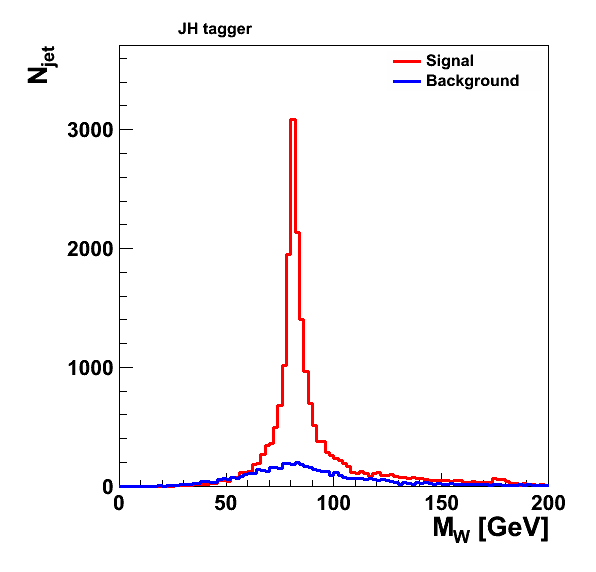
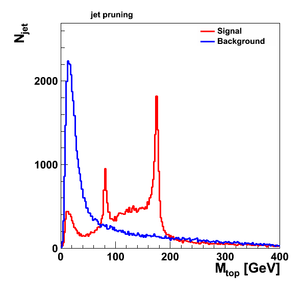
jet pruning (47,016 jets in the signal sample, 52,189 in the background sample):

Higgs Study

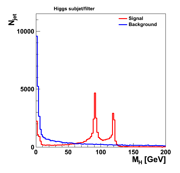
45,260 jets survive the cuts for the signal sample and 56,472 in the background sample.

Cambridge/Aachen 1.2 jets:

After mass-drop filter:

Seattle group

Top study

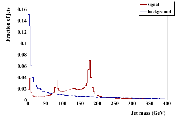
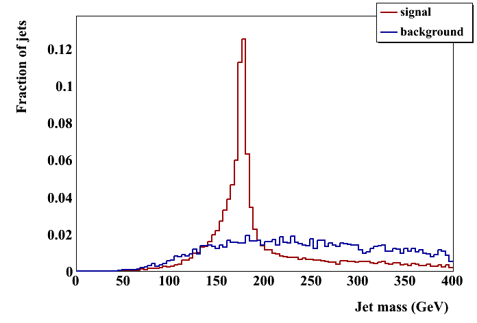
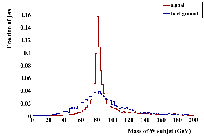
Notes: For the JH and CM taggers, I require maybe_top(). The "top jet" is the sum of all PseudoJets returned by subjets(); the "W jet" is the value of W_subjet(). For pruning and regular C/A I take the "W jet" to be the heavier of the two subjets (found by undoing the last step in the clustering).

I've also attached the SpartyJet scripts I used to generate these plots (minus some ROOT judo I'm also happy to share!). Note that the wiki has attached ".txt" to the file names.

Numbers have been slightly revised: I originally ran CA with R=1.5 to make sure that all constituents were captured; but to be consistent with other groups I have changed to 1.0 for both (likewise below for the Higgs numbers). This means the number of jets after running CA is not the same as after anti-kT. I don't impose another pT cut after running CA.

Total jet numbers:

Anti-kT + pT cut: 47,072 tops 52,201 dijets

CA recluster: 47,114 tops 52.263 dijets

After JH tagger: 19,803 tops 5,278 dijets

After CM tagger: 46,847 tops 51,664 dijets

(Pruning does not remove any jets: same as CA)

Cambridge/Aachen 1.0 jets: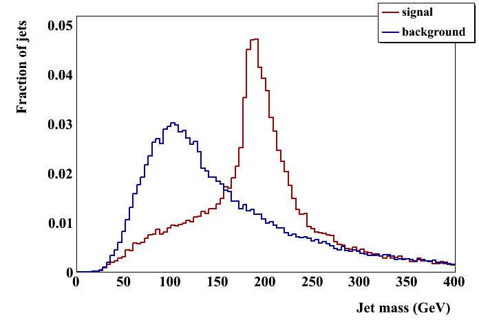

CM tagger (require maybe_top()):

JH tagger (require maybe_top()):

Pruning:

Higgs study

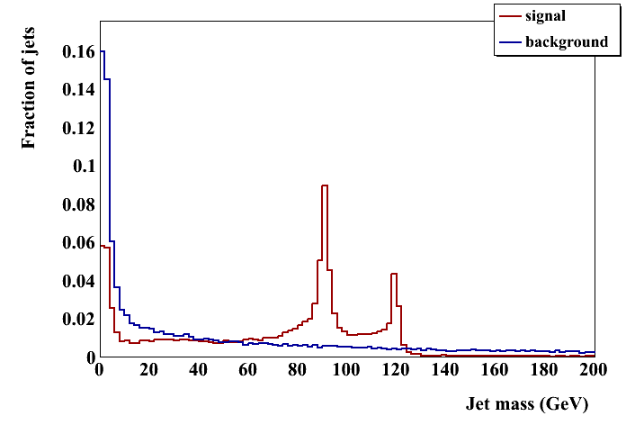
anti-kT + pT cut: 45,260 jets in ZH sample, 56,472 in dijet sample

CA: 45,273 ZH; 56,543 dijet

After mass-drop filter: 44,107 in ZH; 51,552 in dijet

C/A 1.2 jets: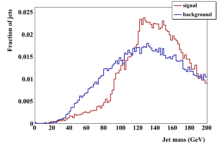

After mass-drop filter:

Davis group

Top study

Signal:

47072 Anti-KT R=1.0 jets with pT>400

47070 Cambridge/Aachen R=1.0 jets with pT>400

Background:

52201 Anti-KT R=1.0 jets with pT>400

52200 Cambridge/Aachen R=1.0 jets with pT>400

Cambridge/Aachen 1.0 jets:

CM tagger

JHU tagger

Pruning (split jet into 2 subjets):

Pruning (split jet into 3 subjets):

Some comparisons for signal jets:

Higgs study

McGill

Top study

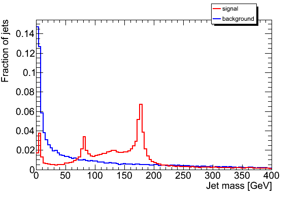
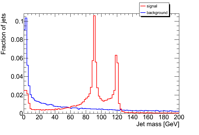
Initial jet finding: 47072 from ttbar, 52201 from dijets

CM: 46805 from ttbar, 51602 from dijets

JH: 19811 from ttbar, 5288 from dijets

PR (requiring >=2 subjets) : 47016 from ttbar, 52189 from dijets

All histograms normalized to unity. 100 bins.

Initial Jet finding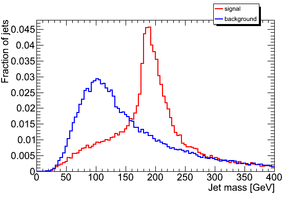

CM

JH

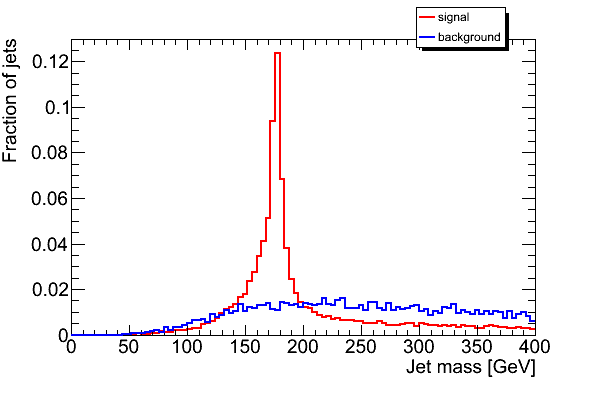
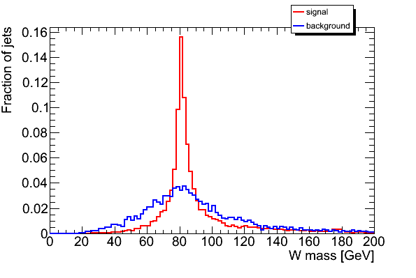Pruning

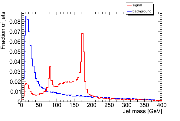
Higgs study

Inital jet finding: Anti-kT 1.2, each jet is reclustered with C/A R=1.5

45260 in ZH, 56472 in Dijet sample

After MDF: 44094 in ZH, 51505 in Dijet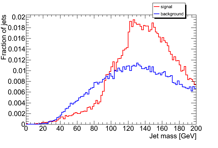

Oxford

Top Study

Ungroomed: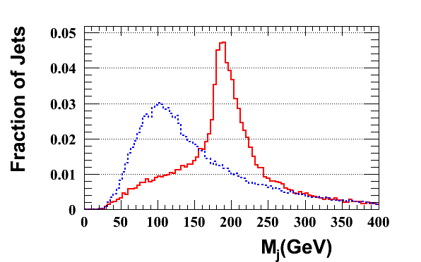

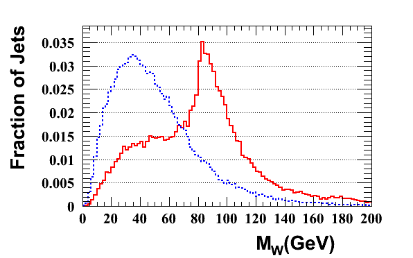JH Tagger:

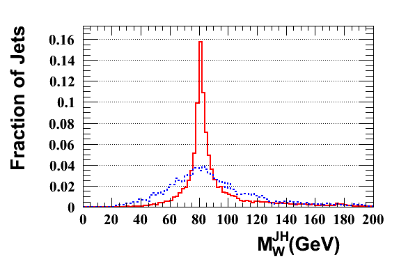CM Tagger:

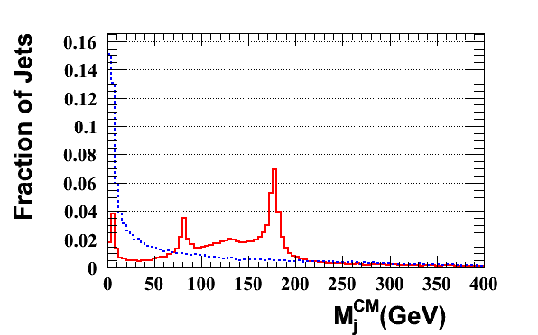
Pruning

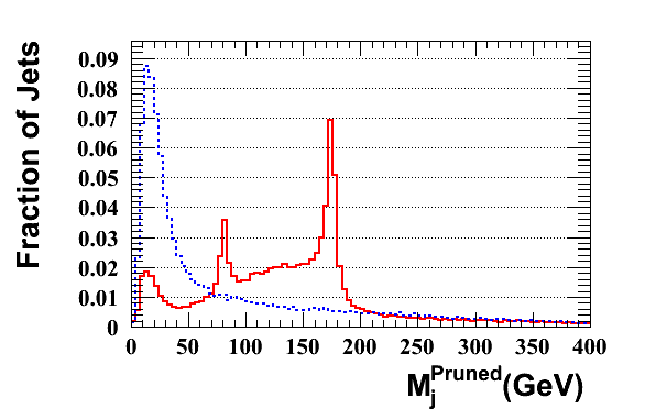
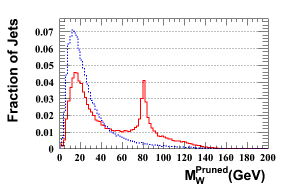
Higgs Study

-- JamesFerrando - 04 Jul 2010

Yale

Top Study

(1) Anti-kT w/ 1.0 + pT > 400: 47072/52201, (2) C/A w/ 1.0 + pT > 400: 47060/52182

JH Tagger: 19806/5265, CM Tagger: 46793/51582

CM Tagger: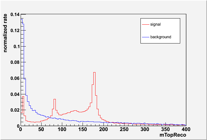

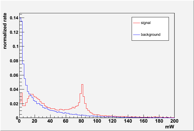JH Tagger:

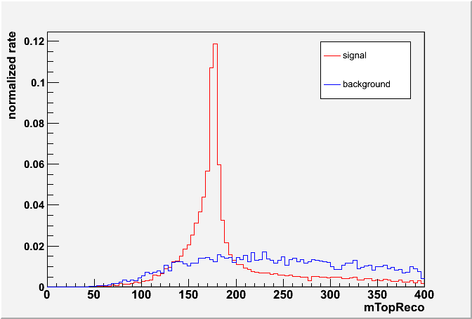
Higgs Study

BDRS Tagger

(1) Anti-kT w/ 1.2 + pT > 200: 45260/56472, (2) C/A w/ 1.2 + pT > 200: 45253/56458, (3) BDRS w/ (0.67, 0.09): 44087/51439

BDRS:

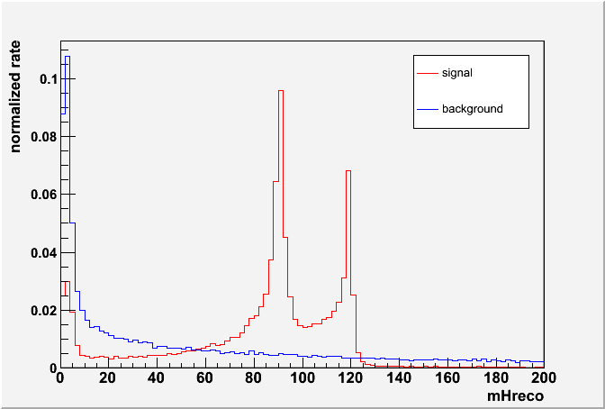
• update 08-19-10 tagrate vs jetpt for eff 35:
  

Gavin

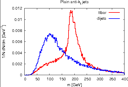
Partial validation results from Gavin (owing to limited time).

Top study

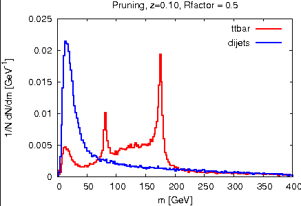
Only top-mass plots are shown and only for the anti-kt jets and for the pruned jets.

Number of jets in the anti-kt sample:

• signal: 47072
• background: 52201

For the C/A sample I've taken just the hardest C/A jet formed from the constituents of each anti-kt jet and not placed any pt cuts on it. Therefore the number of C/A jets (and pruned jets) is identical.